Link Search Menu Expand Document

Textbook Notes

PHIL 120


Table of contents
  1. Chapter 1: Let the Adventure Begin
    1. 1.1: Welcome to the Newsroom
    2. 1.2: Active Learning
    3. 1.3: Logic and Form
    4. 1.4: Entailment = Validity
    5. 1.5: Deductive vs Inductive Logic
  2. Chapter 2: Weird Cases of Validity
    1. 2.1: First Weird Case of Validity
    2. 2.2: Second Weird Case of Validity
    3. 2.3: Third Weird Case of Validity
    4. 2.4: Necessary vs. Contingent
    5. 2.5: Augmentation
  3. Chapter 3: Argument Herooics
    1. 3.1: Identifying Arguments
    2. 3.2: Sentences
    3. 3.3: Soundness and Premise Truth
    4. 3.4: Bivalence
  4. Chapter 4: Meet the Boolean Connectives
    1. 4.1: And here is the conjunction &
    2. 4.2: Or Is it Disjunction v
    3. 4.3: Not to Neglect Negation ~
    4. 4.4: Lost in Translation
  5. Chapter 5: Features of Connectives
    1. 5.1: Scope
    2. 5.2: Arity
    3. 5.3: Advanced Boolean Translations
  6. Chapter 6: Semantics for BOOL - Truth Tables
    1. 6.2: Computing Truth Functions
    2. 6.3: Semantics, Syntax, and Pragmatics
  7. Chapter 7: Using BOOL to Study Reasoning
    1. 7.1: Tautologies and Taut-Falsities
    2. 7.2: Equivalence (DeM and DN)
    3. 7.3: Validity
  8. Chapter 8: BOOLean Algebra
    1. 8.1: Negation Normal Form
    2. 8.2: Chain of Equivalences
    3. 8.3: Distribution Laws
    4. 8.4: Three More laws
  9. Chapter 9: Logic Gates with BOOL
    1. 9.1: Binary Numbers
    2. 9.2: Numerical Truth Tables
    3. 9.3: Electricity
    4. 9.4: BOOLian Logic Gates
    5. 9.5: Building a Computer
  10. Chapter 10: Proofs, Formal and Informal
    1. 10.1: WHat’s a Proof?
    2. 10.2: Informal Proofs
    3. 10.3: Counterexamples
  11. Chapter 11: Formal Proofs
    1. 11.1: &Elim
    2. 11.2: &Intro
    3. 11.3: ~Elim
    4. 11.4: vIntro
    5. Reit
  12. Chapter 12: Proof by Cases
    1. 12.1: Proof by Cases
    2. 12.2: vElim
    3. 12.3: Knights and Knaves
  13. Chapter 13: Reductio
    1. 13.1: Reductio ad absurdum
    2. 13.2: Contradiction Principle
    3. 13.3: #Intro and #Elim
    4. 13.4: ~Intro
  14. Chapter 14: Formal Proof Bootcamp
    1. 14.1: Know the Basics
    2. 14.2: Master Plan - the Main Connective
    3. 14.3: Premises \(\neq\) Conclusions
    4. 14.4: Know Your Premises
    5. 14.5: Know Your Conclusions
    6. 14.6: When All Else Fails: Try Reductio!
  15. Chapter 15: Formal Proofs in BOOL
    1. 15.1: The 5-Step Plan ~(PvQ)
    2. 15.2: Indirect Approach ~(P&Q)
    3. 15.3: Advanced Proof by Cases
    4. 15.4: Advanced Reductio
    5. 15.5: How to Find Shortcuts
  16. Chapter 17: PROP and Conditionals
    1. 17.1: The Condition, \(\to\)
    2. 17.2: The Biconditional, \(\iff\)
    3. 17.3: Difficult Translations
    4. 17.4: Truth Tables for Conditionals
  17. Chapter 18: Proofs with Conditionals
    1. 18.1: Modus Ponens
    2. 18.2: \(\to\) Elim and \(\iff\) Elim
    3. 18.3: Conditional Proof
    4. 18.4: \(\to\) Intro and \(\iff\) Intro
  18. Chapter 19: Formal Proofs in PROP
    1. 19.1: \(\to\) Conclusions
    2. 19.2: \(\to\) Premises
    3. 19.3: The Contradiction Tricky
    4. 19.4: The Reiteration Trick
    5. 19.5: Biconditionals
  19. Chapter 20: Metalogic
    1. 20.1: Soundness and Completeness
    2. 20.2: Proving Soundness
    3. 20.3: Truth-Functional Completeness
    4. 20.4: More TFC
    5. 20.5: Nor and Nand
  20. Chapter 21: Welcome to FOL
    1. 21.1: Terms - Constants and Variables
    2. 21.2: Predicates - Properties and Relations
    3. 21.3: The Identity Predicate
    4. 21.4: Atomic Sentences
  21. Chapter 22: Meet the Quantifiers
    1. 22.1: All (A) and Exists (E)
    2. 22.2: Variables, Free and Bound
    3. 22.3: Well-Formed Formulas (WFFs) vs Sentences
  22. Chapter 23: Semantics of FOL
    1. 23.1: Names and Objects
    2. 23.2: The Domain
    3. 23.3: Predicates and Intended Interpretations
  23. Chapter 24: Aristotelian Forms
    1. 24.1: Four Aristotelian Forms
    2. 24.2: Advanced Forms
    3. 24.3: Vacuous Generalizations
    4. 24.4: Pairs of Contradictories
  24. Chapter 25: FOL Equivalences
    1. 25.1: Demorgan’s for Quantifiers
    2. 25.2: Null Quantification
    3. 25.3: Variable Switch
    4. 25.4: Distribution for Quantifiers
    5. 25.5: Prenex Normal Form and Chain of Equivalences
    6. 25.6: Quantifier Reorder
  25. Chapter 26: FO Necessities
    1. 26.1: FO Validities
    2. 26.2: FO Falsities
    3. 26.3: Truth-Functional Form Algorithm
    4. 26.4: The Chart
  26. Chapter 27: Counterexamples in FOL
    1. 27.1: Counterexamples in FOL
  27. Chapter 28: Multiple Quantifiers
    1. 28.1: Same Quantifiers
    2. 28.2: Mixed Quantifiers
  28. Chapter 29: Numerical Quantification
    1. 29.1: At Least
    2. 29.2: At Most
    3. 29.3: Exactly
    4. 29.4: Definite Descriptions - ‘The’
  29. Chapter 30: Proofs in FOL - 2 Easy Ruels
    1. 30.1: Simple Informal Proofs
    2. 30.2: \(\exists\)Intro - Existential Generalization
    3. 30.3: \(\forall\)Elim - Universal Instantiation
  30. Chapter 31: Proofs in FOL - 2 Hard Rules
    1. 31.3: Universal Generalization
    2. 13.2: \(\forall\) Intro
    3. 13.3: Existential Instantiation
    4. 13.4: \(\exists\)Elim
  31. Chapter 32: = Proofs
    1. 23.1: =Elim
    2. 23.2: =Intro
  32. Chapter 33: FOL Proofs
    1. 33.1: Universals
    2. 33.2: Existentials
    3. 33.3: Key Pattern ~\(\exists\)xP(x)
    4. 33.4: Annoying Pattern ~\(\forall\)xP(x)
    5. 33.5: Regular Routine for Quantifiers
  33. Chapter 34: Logic and Set Theory
    1. 34.1: Sets and Membership
    2. 34.2: Cardinality = Size
    3. 34.3: Natural Numbers and Infinite Sets
    4. 34.4: 1-to-1 Correspondence, Transfinite Arithmetic
  34. Chapter 35: Logic and Infinity
    1. 35.1: E, O, Z
    2. 35.2: The Rational Numbers Q
    3. 35.3: The Real Numbers R

Chapter 1: Let the Adventure Begin

1.1: Welcome to the Newsroom

  • Logic is the rules and principles of reasoning we use every day.
  • Logic can also mean the study of our reasoning.
  • Formal logical systems/logical systems: a model we create to study our reasoning.

1.2: Active Learning

  • Humans learn best by doing.
  • Tabula rasa vs constructivism
  • Constructivism: Students must actively build their understanding of the material..

1.3: Logic and Form

  • We study the form/structure of reasoning an dinferences.
  • Structure is a repeatable pattern.
  • Replacing words with symbols allows us to reveal forms.
  • Reasoning depends on form.

1.4: Entailment = Validity

  • In logic, we want to know when some logic guarantees something is true.
  • Deductive logical entailment/entailment.
  • A set of premises entails a conclusion if whenever the premises are true, the conclusion is also true.
  • A valid argument: the premises entail the conclusion.

1.5: Deductive vs Inductive Logic

  • Inductive logic: probability and likelihood.
  • Deductive logic: guarantee and certainty.
  • Principle of Charity: give people the benefit of the doubt and interpret their arguments in a reasonable way, if possible.

Chapter 2: Weird Cases of Validity

2.1: First Weird Case of Validity

  • Circular reasoning: the prmeise and conclusion are the same.
  • All circular reasoning is valid: if the premise is true, so is the conclusion.
  • Circular reasoning is any case of assuming what you are trying to prove.
  • Fallacy: a tempting but flawed form of reasoning.
  • Whether circular reasoning is good or bad depends on the circumstances one is in.

2.2: Second Weird Case of Validity

  • Reasoning from a contradiction is valid.
  • Contradiction - occurs when two sentneces say the opposite of each other.
  • Contradiction - a logical falsehood, a sentence that is necessarily false.
  • Contradictory set - a group of sentences that can’t be true at once.
  • Any argument with contradictory premises is valid.
  • Validity says that whenever all premises are true, the conclusion must be true. Contradictory premises satisfy this definition trivially because the premises can never be true.
  • The only way to show that an argument is invalid is to find a way to make the premises true but the conclusion false.

2.3: Third Weird Case of Validity

  • A set of premises can be empty. We can still use the definition of validity to assess the argument.
  • If there are no premises, the conclusion must always be true.
  • We can cehck the validity of an argument with an empty set of premises by checking if the conclusion is necessarily true.
  • Logical turth -a sentence that is necessarily true because of the laws of logic.
  • An argument with a logically true conclusion is always valid.

2.4: Necessary vs. Contingent

  • Some statements are neither necessarily true or necessarily false.
  • The opposite of necessary is contingent - something that may or may not be true.
  • Necessary truths may manifest in a wide variety of laws and backgrounds.

2.5: Augmentation

  • Augmentation: to add one or more premises to make an argument a new argument.
  • When we augment a valid argument, the new premise may add relevant or irrelevant information. It may also contradict existing premises - but the argument will always remain valid.
  • Induction - a set of premises may support or confirm a conclusion.
  • Validity is a tipping point. once information guarantees the conclusion is true, you cannot destroy validity by adding information - only by taking the information away.

Chapter 3: Argument Herooics

3.1: Identifying Arguments

  • Identifying arguments can be surprisingly difficult.
  • Argument: premises and conclusion.
  • Premise signals: words that indicate a premise. “Because”, “since”, “for”, “given”.
  • Conclusion signals: words that indicate a conclusion. “Thus”, “so”, “hence”, “therefore”.

3.2: Sentences

  • Anything that can carry information can be studied with logic.
  • Sentences can be short in pithy; some ask questions; some make comma ds.
  • We care interested in assertions or statements: sentences that make cleaims.
  • Sentences int he context of logic have truth values.

3.3: Soundness and Premise Truth

  • Validity doesn’t care about actual truth values; it is a hypothetical/conditional property.
  • Truth concerns the relationship between premises and the world.

3.4: Bivalence

  • Truth and falsity: truth values.
  • In logical systems studied in this course, there are only two possible truth values (True and False).
    • These are bivalent logics.

Chapter 4: Meet the Boolean Connectives

4.1: And here is the conjunction &

  • BOOL: a logical system, short for Boolean logic.
  • & is only allowed to connect two entences together; we technically shouldn’t say P&Q&R but we can infer an order of operations.
  • If English groups sentences clearly, we need to also group them in bool.
  • & - conjunction, ampersand, and
  • Sentences are atomic sentences/atoms - they are the building blocks of BOOL.
  • Complex sentences are combinations of atomic sentneces.

4.2: Or Is it Disjunction v

  • Disjunction, wedge, or: v.
  • Disjunction is connective; we can use long strings of disjunctions.
  • Conjuncts and disjuncts

4.3: Not to Neglect Negation ~

  • The third connective is ~: negation, tilde, not.
  • These three connectives are the Boolean connectives.
  • Preserve as much structure whne translating into BOOL as possible.
  • Negation always applies to the smallest possible scope of sentence.
  • Scope - how much of a sentence a connective governs.
  • Default: negation has a narrow scope.

4.4: Lost in Translation

  • Some bits are lost in translation.
  • BOOl helps us study how we reason.
  • When we translate a complex sentence into BOOL, we need to capture logical commitmnets.

Chapter 5: Features of Connectives

5.1: Scope

  • Scope is the extent of a connective - how much of a sentence it governs.
  • Each occurrence of a connective has its own scope.
  • Main connective - the connective with wide scope, governs the whole sentence

5.2: Arity

  • Arity: the number of inputs a connective takes.
  • If a connective takes only one input, it is unary. If it takes two inputs, it is binary.

5.3: Advanced Boolean Translations

  • ‘Neither Pia nor Quinn is guilty’. ~P&~Q or ~(PvQ)
  • You can translate neither/not in two ways.
  • When connectives are the same time, we can allow chaining because any way of grouping yields the same result. (P&Q)&R = P&(Q&R).
    • This property does not hold for mixed connectives.
  • When you have mixed binary connectives and English doesn’t group them, you must give both translations until you know which is correct.
  • Ambiguity - when a word or sentence has two different but possible meanings.

Chapter 6: Semantics for BOOL - Truth Tables

  • Truth tables: charts showing every possible way a sentence could be true or false.
  • Truth table for an atomic sentence \(P\):
P
T
F
  • Truth functionality: the truth value of any complex sentence is dependent on the truth values of the atomic sentences it is comprised of.
P~P
TF
FT
  • Canonical form: reference columns are alphabetical; the patterns of Ts and Fs are awlays the same.
PQP&Q
TTT
TFF
FTF
FFF
PQPvQ
TTT
TFT
FTT
FFF

6.2: Computing Truth Functions

  • BOOL has only three connectives; all are truth functional.
PQ~Pv(Q&P)
TT?
TF?
FT?
FF?
  • We begin by computing the inputs to the disjunction, which is the main connective.
PQ~PQ&P~Pv(Q&P)
TTFT?
TFFF?
FTTF?
FFTF?
  • Now, we can fill in the disjunction.
PQ~PQ&P~Pv(Q&P)
TTFTT
TFFFF
FTTFT
FFTFT
  • The number of rows in any table is \(2^n\), where \(n\) is the number of atomic sentences.

6.3: Semantics, Syntax, and Pragmatics

Semantics = meaning.

Syntax = grammar.

Pragmatics = use.

Chapter 7: Using BOOL to Study Reasoning

7.1: Tautologies and Taut-Falsities

  • An atomic sentence P might be true or false, but the complex sentence Pv~P cannot possibly be flase.
  • Tautologies - logical truths, a sentence that is logically true because of the truth-functional connectives.
    • Can be identified when a sentence’s truth table has all Ts.
  • Pv~P - law of the excluded middle; there is no third option or middle ground.
  • Tautological falsities: a sentence with all Fs in its truth function.
  • Tautologically contingent: a sentence with at least one T and F.

7.2: Equivalence (DeM and DN)

  • Equivalence - two sentences already have the same truth value; they co-vary in truth value.
  • Tautologically equivalent: sentences that are equivalent because of the truth-functional connectives.
  • DeMorgan’s Laws: ~(PvQ) ⇔ ~P&~Q, ~(P&Q) ⇔ ~Pv~Q.
  • ⇔ is shorthand for ‘logically equivalent’.
  • Object language - formal language defined as part of the logical system.
  • Metalanguage - language defined to talk about the language.
  • Law of Double Negation: P ⇔ ~~P.

7.3: Validity

  • When all the premises are true, the conclusion must also be true.
  • Truth Table method: build a joint truth table to assess an argument for validity.
  • Counterexample: a row on which the premises are true and the conclusion false.

Chapter 8: BOOLean Algebra

8.1: Negation Normal Form

  • Negation Normal form: any negations are in narrow scope.
  • When a sentence is in NNF, the basic units are atomic sentences and negations of atomic sentences combined with disjunctions and conjunctions.
  • Literals: atomic sentences and negations of atomic sentences.

8.2: Chain of Equivalences

  • You can keep simplifying an expression using DeMorgan’s laws and Double Negation.
~(PvQ) ⇔ ~P&~Q

~(P&Q) ⇔ ~Pv~Q

P ⇔ ~~P
  • You must only use one principle at a time.
  • Chain of equivalences: continuous transformations and simplifications as a result of DN and DeM.
~~~(~~(~P&~Q)v~(~R&~S))
⇔ ~((~P&~Q)v~(~R&~S))   DN
⇔ ~(~P&~Q)&~~(~R&~S)    DeM
⇔ ~(~P&~Q)&(~R&~S)      DN
⇔ ~(~P&~Q)&(~R&~S)      DeM
⇔ (PvQ)&(~R&~S)         DeM

8.3: Distribution Laws

  • Distribution laws:
Pv(Q&R) ⇔ (PvQ)&(PvR)

P&(QvR) ⇔ (P&Q)v(P&R)
  • Distribution changes the number of atomics in a sentence, but DeMorgan’s doesn’t.
  • DeMorgan’s law is best thought of as ‘flipping’ a conjunction to a disjunction and vice versa.
  • Sometimes, you need to distribute with larger ‘chunks’. For instance, you can distribute (A&B)v in (A&B)v(C&D) to form ((A&B)vC)&((A&B)vD).
  • After we distribute conjunctions and disjunctions, we don’t have disjunctions with wide scope around conjunctions.

8.4: Three More laws

  • BOOL obeys laws that have algebraic counterparts.
  • Associativity
(P&Q)&R ⇔ P&(Q&R)

(PvQ)vR ⇔ Pv(QvR)
  • Commutativity
P&Q ⇔ Q&P

PvQ ⇔ QvP
  • Idempotence:
P&P ⇔ P

PvP ⇔ P

Chapter 9: Logic Gates with BOOL

9.1: Binary Numbers

  • Bases: changing the number of things that can be represented with a single ‘digit’ or ‘place’.
  • Binary - a base-two system. Two numerals represent every number.

9.2: Numerical Truth Tables

  • We can associate 1 = True and 0 = False.
  • The number of rows in a truth table is fixed by the number of atomic sentences - two to the power of the number of atomics.

9.3: Electricity

  • Atomic sentence: Gate down/closed = on = true = 1.
  • Switch down/closed = Atomic True
  • Switch up/open = Atomic False
  • Bulb on = Complex True
  • Bulb off = Complex False
  • Series: gates on the same piece of wire. Gates in series always means conjunction - they must all be closed for electricity to flow.

9.4: BOOLian Logic Gates

  • Parallel gates - when gates are separated on different pieces of wire. Parallel gates are represented by disjunctions.
  • Negation - moving the contact such that an ‘open position’ completes the circuit.

9.5: Building a Computer

  • One of the fundamental jobs of a computer processor is adding numbers.
  • Bit - a binary digit of infromation.
  • We need to wire a machine that computes the following:
XYAnswer
111 0
100 1
010 1
000 0
  • We can use a sum and carry:
XYCarrySum
1110
1001
0101
0000
  • Sum is XOR: exclusive disjunction. (P&~Q)v(~P&Q) or (PvQ)&~(P&Q).

Chapter 10: Proofs, Formal and Informal

10.1: WHat’s a Proof?

  • Proof: a step-by-step explanation from which something necessarily does or does not follow.
  • Proof: a demonstration that an argument is valid or invalid.
  • A proof is not an argument.
  • Proofs can be good or bad, successful or unsuccessful.
  • Steps in a proof must be obvious and valid for a proof to be good.
  • Formal proofs: written in BOOL.
  • Informal proofs: written in English.

10.2: Informal Proofs

  • Intermediary conclusion: the conclusion of one of the inferential steps used to reach the final conclusion.
  • Common parts of a proof:
    1. Opening: stating “proof” at the start to clarify what you’re doing.
    2. Restating a premise.
    3. Justifying an inference.
    4. Stating an intermediary conclusion.
    5. Stating the final conclusion.
    6. Closing: stating “done” or “Q.E.D.” or ∎.
  • Q.E.D. - Latin, ‘Done’. ∎ - tombstone symbol.
  • A proof does not need to use every premise in the argument.

10.3: Counterexamples

  • A proof can show that an argument is invalid via the counterexample.
  • Counterexmaple: a specific case showing the premises can be true and the conclusion false.
  • All proofs of invalidity start with “Proof by counterexample.”

Chapter 11: Formal Proofs

11.1: &Elim

  • Final feature we will add to BOOL: a formal proof system.
  • Formal proof: a table with three columns that follows certain rules.
  • First column: numbers; second: BOOL sentneces; third: citations/justifications.
  • Premise - justifies premises.
  • &Elim - conjunction elimination. How to use or eliminate a wide-scope conjounction.
  • When you use &Elim, you must cite exactly one sentence; a semicolon goes between the rule name and the line number it cites.
  • All formal proof rules only apply to the main connective.

11.2: &Intro

  • &Intro can be used to ‘introduce’ a conjunction.
  • Conjunction always requires two sentences. &Intro must cite two lines.
1. P     Premise
2. Q     Premise
3. Q&P   &Intro;1,2

11.3: ~Elim

  • You can use ~Elim to eliminate two negations together.
1. Q&~~R   Premise
2. Q       &Elim;1
3. ~~R     &Elim;1
4. R       ~Elim;3
5. Q&R     &Intro;2,4

11.4: vIntro

  • You can use vIntro to introduce disjunction operations.
1. ~~P&~~~Q  Premise
2. ~~~Q      &Elim;1
3. ~Q        ~Elim;2
4. Rv~Q      vIntro;3
  • You can add complex sentences as disjuncts.

Reit

  • Reit: reiteration. Allows you to repeat the previous line.
  • Reit is always valid because if circular reasoning.
1. P    Premise
2. P    Reit;1
3. P&P  &Intro;1,2

Chapter 12: Proof by Cases

12.1: Proof by Cases

  1. Start by saying “Proof by cases”.
  2. Restate the disjunction you are using to structure the proof aroudn.
  3. Create a case for each disjunct in the disjunction.
  4. “Case 1: Assume…”
  5. “Case 2: Asume…”
  6. Prove that the same conclusion follows in each case.
  7. “So we know that [the conclusion] follows in every case. Done.”

12.2: vElim

  • vElim is the formal proof rule that goes with proof by cases.
  • vElim works like proof by cases; we need to formally model temporary assumptions for each case.
  • Subproof: a mini proof inside of a main proof.
1. PvQ     Premise
2. | P     Assume
3. | QvP   vIntro;2
4. | Q     Assume
5. | QvP   vIntro;4
6. QvP     vElim;1,2-3,4-5

12.3: Knights and Knaves

  • Solving Knights and Knaves problems via proof by cases.
  • x is a knight or knave, or y is a knight or knave. Temporarily assuming x is a knight/knave, what holds true?

Chapter 13: Reductio

13.1: Reductio ad absurdum

  • ~Intro is paired with an informal proof method that pairs it. Proof by contradiction, reductio ad absurdom, reductio.
  • ~Intro and Reductio: how to reason to a negation, formally and informally.
  • If you can make a temporary assumption and show that a contradiction results, then you know that ~assumption is true.
  • Constructing reductio proofs:
    1. Start with “proof by contradiction/reductio.”
    2. Write “assume for reductio …, we want to show a contradiction results.”
    3. Demonstrate how a contradiction results.
    4. Write “hence we know … by reductio. Done.”

13.2: Contradiction Principle

  • Tautological contradiction: # or ⊥, always F/0.
  • # is a sentence, not a connective. It can appear in complex sentences: P&# or ~#.
  • Disjoining with a tautological falsity returns the same truth sentence as the original sentence.
  • A contradiction entails anything.
P&~P ⇒ R
Q&~Q ⇒ R
# ⇒ R

P&~P ⇒ P&~P
Q&~Q ⇒ Q&~Q
# ⇒ #

P&~P ⇒ Q&~Q
P&~P ⇒ #
# ⇒ P&~P
  • Contradiction principle: only a contradiction can entail a contradiction.
  • TO prove an argument by reductio, we assume ~ conclusion and show that the premises and conclusions \(\to \bot\).
1. If Q, then P
2. ~P
Thus,
3. ~Q

13.3: #Intro and #Elim

  • Only a contradiction can entail #, any contradiction can entail #.
1. P      Premise
2. ~P     Premise
3. #      #Intro;1,2
  • To introduce a tautological falsity, establish a sentence and its negation. These sentences do not necessarily need to be atomic.
  • #Elim: how to use a symbol that you already have. A contradiction entails anything. If you have a #, you can write anything you want and cite #Elim. (Easiest rule ever.)

13.4: ~Intro

  • ~Intro allows us to make a wide-scop enegation.
  • To prove ~P, we temporarily assume P and prove #.
  • ~Intro = Reductio.
1. ~(PvQ)      Premise
2. | P         Assume
3. | PvQ       vIntro;2
4. | #         #Intro;1,3
5. | ~P        ~Intro;2-4
  • Cite a subproof where you assume the opposite of your conclusion. There is not a specific line to cite.
1. ~(P&Q)      Premise
2. P           Premise
3. | Q         Assume
4. | P&Q       &Intro;2,3
5. | #         #Intro;1,4
6. ~Q          ~Intro;3-5

Chapter 14: Formal Proof Bootcamp

14.1: Know the Basics

  • Obey parentheses.
  • ~Elim does not work exactly like the Double Negation principle - you can only eliminate two negations at a time.
  • vElim and ~Intro are the only rules that allow you to get out of a subproof into a parent proof.
  • Never start a subproof without a plan.
  • In vElim, do cases from left to right.
  • You need to do a subproof for every case.
  • One-line subproofs don’t need an indented dash.

14.2: Master Plan - the Main Connective

  • Look at the main connectives. Intro and Elim rules only apply to the main connective of a sentence.

14.3: Premises \(\neq\) Conclusions

  • What you do with a main connective depends on whether it is a premise or a conclusion.
  • Elim rules eliminate a connective: apply to premises.
  • Intro rules introduce a connective: apply to conclusions.

14.4: Know Your Premises

  • & premise - bring down conjuncts.
  • v premise - start proof by cases by assuming a disjunct.

14.5: Know Your Conclusions

  • & conclusion - prove each conjunct, then build up with &Intro
  • v conclusion - create from one side with vIntro
  • ~ conclusion - do a reductio with ~Intro

14.6: When All Else Fails: Try Reductio!

  • Sometimes reductio is the right idea, even if the conclusion isn’t a wide-scope negation.

Chapter 15: Formal Proofs in BOOL

15.1: The 5-Step Plan ~(PvQ)

  • Strategy - look at main connectives.
1. ~(PvQ)       Premise
2. P            Assume
3. PvQ          vIntro;2
4. #            #Intro;1,3
5. ~P           ~Intro;2-4
  1. Pick a disjunct
  2. Put it in a subproof
  3. Build the disjunction
  4. Introduce the contradiction
  5. Finish the reductio

15.2: Indirect Approach ~(P&Q)

  • Apply the five step plan inside a reductio by using ~(P&Q) \(\to\) assume ~(~Pv~Q).

15.3: Advanced Proof by Cases

  • Nested proof by cases - one proof by cases inside the other.

15.4: Advanced Reductio

  • Reductio gives us another sentence to work from.
  • To prove a tautology in BOOL (no premises), you always begin with reductio.
1. | ~(Pv~P)     Assume
2. || P          Assume
3. || Pv~P       vIntro;2
4. || #          #Intro;1,3
5. | ~P          ~Intro;2-4 
6. | Pv~P        vIntro;5
7. | #           #Intro;1,6
8. Pv~P          ~Intro;1-7
  • Never assume what you already know.

15.5: How to Find Shortcuts

  • Shortcuts involve noticing a recurring pattern, and let you find a faster and more elegant way to do the proof.

Chapter 17: PROP and Conditionals

17.1: The Condition, \(\to\)

  • BOOL is a powerful tool - it can prove the validity of any argument valid on account of conjunction, disjunction, and engation.
  • BOOl is limited.
  • PROP: an extension of BOOL, including everything and adding \(\to\) and \(\iff\).
  • \(\to\) - conditional, arrow, if/then.
  • Conditionals: assert a conditionality between two things. Also known as: hypotheticals.
  • “if”: antecedent. “then”: consequent.
  • \(P \to Q\) is not a causal claim; it just claims that if \(P\) is true, then \(Q\) is true too.

17.2: The Biconditional, \(\iff\)

  • Biconditional: two conditionals.
  • “if and only iff”/”iff” - \(P\iff Q = P\to Q & Q \to P\)
  • iff is not redundant
  • \(P\) just in the case of \(Q\) - \(P \iff Q\).

17.3: Difficult Translations

  • Necessary and sufficient conditions are conditional claims.
  • If X is sufficient for Y, then X \(\to\) Y.
  • If X is necessary for Y, then Y \(\to\) X.

17.4: Truth Tables for Conditionals

  • Conditionals are truth functional. Evaluate whether the condition is true or not given the truth values of the atomic sentences.
  • A conditional with a false antecdent is trivially true, because the initial conditional is false.
  • Contrapositive: P \(\to\) Q \(\iff\) ~Q \(\to\) ~P
  • PROP does not give us the ability to express more truth functions than BOOL.
  • However, PROP allows us to model and study conditionals.

Chapter 18: Proofs with Conditionals

18.1: Modus Ponens

  • PROP has all the formal rules that BOOl does - but we need Intro and Elim for conditional and biconditional rules.
  • Reasoning from a conditional is very natural.
  • Modenus ponens: from \(P\) and if \(P\) then \(Q\), you can infer \(Q\).
  • Affirming the consequent: \(P \to Q\) and \(Q\); therefore, \(P\). This is a fallacy.
  • With bidirectional conditions, you can do Modus Ponens in either direction.

18.2: \(\to\) Elim and \(\iff\) Elim

1. P        Premise
2. P -> Q   Premise
3. Q        ->Elim;1,2

18.3: Conditional Proof

  • Conditional obeys transitivity: \(P \to Q\) and \(Q \to R\) entail \(P \to R\).
  • You always want to show that when the antecedent is true, the consequent is true.
  • For biconditionals, do two separate proofs in either direction.

18.4: \(\to\) Intro and \(\iff\) Intro

  • Conditional proof: temporarily assume the atecedent, get the consequent.
  • Setting up an \(\to\)Intro proof is the easiest way to prove a conditional.

Chapter 19: Formal Proofs in PROP

19.1: \(\to\) Conclusions

  • When your conclusion is a wide-scope arrow, begin with an \(\to\)Intro proof. This is always the best way to go about it.

19.2: \(\to\) Premises

  • A conditional premise does not tell you what to do right away.
  • You must ‘earn’ the antecedent

19.3: The Contradiction Tricky

  • A negation around a conditional can be tricky.
1. ~(P->Q)         Premise
2. | ~P            Assume
3. || P            Assume
4. || #            #Intro;2,3
5. || Q            #Elim;4
6. | P->Q          ->Intro;3-5
7. | #             #Intro;1,6
8. P               ~~Intro;2-7

19.4: The Reiteration Trick

1. ~(P->Q)     Premise
2. | Q         Assume
3. || P        Assume
4. || Q        Reit;2
5. | P->Q      ->Intro;3-4
6. | #         #Intro;1,5
7. ~Q          ~Intro;2-6

19.5: Biconditionals

  • Biconditionals are the same, just do the work twice.
1. ~(P<->Q)    Premise
2. | P&Q       Assume
3. || P        Assume
4. || Q        &Elim;2
5. || Q        Assume
6. || P        &Elim;2
7. | P<->Q     <->Intro;3-4,5-6
8. | #         #Intro;1,7
9. ~(P&Q)      ~Intro;2-8

Chapter 20: Metalogic

20.1: Soundness and Completeness

  • Metalogic: the study of logical systems.
  • We can ask metalogical questions about whether truth-tables and formal proofs always deliver the same result.
  • Well-designed logical systems should satisfy this above property.
  • We want to prove two properties:
    1. Soundness. If we can give a formal proof of an argument, it is valid by the truth-table method.
    2. Completeness. If an argument is valid (by the truth table method), then we can give a formal proof for it.

20.2: Proving Soundness

  • Any argument we can give a formal proof of in bool is valid.
  • Soundness is a conditional claim.
  • 1-step soundness: if a conclusion can be proven in BOOL with a one-step formal proof, then that conclusion really is a logical consequence of the premises.
  • vElim and ~Intro cannot be used to justify the conclusion because they take more than one line.

20.3: Truth-Functional Completeness

  • TFC: the ability to express any possible truth function.
  • TFC concerns the expressive power of aysstem.
  • All sentences of BOOL are finitely long.
  • Classical logics: logical systems created with standard properties like bivalence and finitely long sentences.
  • TFC algorithm: creating a sentence of BOOL expressing a truth function, regardless of the truth function.
  • Disjoin the exact conditions for each truth value.

20.4: More TFC

  • We can prove that PROP is truth functionally complete.
  • Something can be TFC with ‘less’ than BOOL.
  • We only need two connectives, either negation or disjunction and negation.
  • \({\to, ~}\) is TFC
  • \({\iff, ~}\) is not TFC
  • None of the connectives alone is TFC

20.5: Nor and Nand

  • \(\downarrow = ~v\); NOR - not or, FFFT truth table.
  • | = ~&; NAND - not and, FTTT truth table.
  • NAND and NOR can express conjunction and negation. NAND and NOR are therefore TFC alone.

Chapter 21: Welcome to FOL

21.1: Terms - Constants and Variables

  • FOL: First-order Logic.
  • Quantifiers in the logic range over sets of objects in the domain, rather than sets of sets of objects.
  • IN BOOl and PROP, the smallest units of language are atomic sentences.
  • Atomic sentences can have parts.
    • Terms - objects.
      • Constants (names)
      • Variables
  • Names in FOL - constants; pick out the same thing.
  • Variables can refer to different things.

21.2: Predicates - Properties and Relations

  • Predicates - how we say things about objects.
  • Predicates must start with a capital letter.
  • Argument places - gaps in the predicate where we insert terms.
  • Number of argument places - arity.
  • Order of the argument places matters
  • Properties - predicates with one argument place.
  • Relations - predictes with two or more argument places.

21.3: The Identity Predicate

  • Identity - =.
  • infix - go in the middle of terms.
  • prefix - go before terms
  • Identity has three important properties - reflexible, symmetric, transitive

21.4: Atomic Sentences

  • The correct number of names depends on the arity of the predicate

Chapter 22: Meet the Quantifiers

22.1: All (A) and Exists (E)

  • Quantifier - a part of language for referring to a quantity of things
  • Logical symbol for all - \(\forall\)
  • All objects are fish - \(\forall \text{xFish(x)}\)
  • \(\exists\) - Existential Quantifier. Makes a claim of existence.

22.2: Variables, Free and Bound

  • Constants refer to the same object
  • Variables aren’t assigned a specific interpretation.
  • Examples:
    • Something is a dog. \(\exists \text{Dog}(x)\)
    • Everything is a dog. \(\forall \text{Dog}(x)\)
    • Some cat likes some dog. \(\exists x \exists y (\text{Cat}(x) & \text{Dog}(y) & \text{Likes}(x, y))\)
  • When a quantifier connects with a variable, it binds the variable.
  • When a variable is not bound it is free.

22.3: Well-Formed Formulas (WFFs) vs Sentences

  • FOL is bivalent; every sentence has exactly one truth value.
  • New grammatical category - an open formula, a formula with a free variable in it.
  • If a formula has no free variable, then it is a closed formula (i.e. a sentence).
  • Well-formed formulas (WFF): open and closed formulas

Chapter 23: Semantics of FOL

23.1: Names and Objects

  • Rule of names - each name represents one object.
  • Each name does not need to pick out a different object.

23.2: The Domain

  • Domain - the set of objects a quantifier ranges over
  • If you have multiple quantifiers in a sentence or multiple sentences in an argument, thye must all operate on the same domain. If this prerequisite is not met, fallacious reasoning is allowed.

23.3: Predicates and Intended Interpretations

  • Identity predicate = - only predicate that gets its own logical symbols.
  • Logical symbols are fixed parts of the system.
  • Intended Interpretation

Chapter 24: Aristotelian Forms

24.1: Four Aristotelian Forms

  • Aristotelian form - “All Ps are Q”
All dogs are running.
Ax(D(x)->R(x))
  • Aristotelian form - “Some Ps are Q”
Some dogs are running.
Ex(D(x)&R(x))
  • Boolean Definition of Conditional (BDC): Ex(~P(x)vQ(x))
    • Does not say some Ps are Q
    • Abdominable form: never translate anything with \(\exists x\) around \(\to\).
  • Aristotelian form: “No Ps are Q”
No dogs are running.
~Ex(D(x)&R(x))
Ax(D(x)->~R(x))

All forms:

All Ps are Q: Ax(P(x)->Q(x))
Some Ps are Q: Ex(P(x)&Q(x))
No Ps are Q: Ax(P(x)->~Q(x)) or ~Ex(P(x)&Q(x))
Some Ps are not Q: Ex(P(x)&~Q(x))

24.2: Advanced Forms

All happy dogs are running.
Ax((D(x)&H(x))->R(x))
  • When translating complex forms, formulas can be messy.
  • Drop parentheses when you can.

24.3: Vacuous Generalizations

  • When there are no \(P\)s, then “All \(P\)s are \(Q\)” is vacuously true.

24.4: Pairs of Contradictories

  • Contradictories - sentences that say the opposite of each other.

Chapter 25: FOL Equivalences

25.1: Demorgan’s for Quantifiers

~AxP(x) ⇔ Ex~P(x)
~ExP(x) ⇔ Ax~P(x)

25.2: Null Quantification

  • If a quantifier doesn’t bind to any variables in the formula, it is null on it.
  • If a quantifier is null on a formula, the quantifier is always put on wide scope.
P&AxQ(x) ⇔ Ax(P&Q(x))

25.3: Variable Switch

  • Variable Switch: you can uniformly substitute one variable for another.
AxP(x) ⇔ AyP(y)
ExP(x) ⇔ EyP(y)
  • Restrictions
    • All occurrences of the variable connected to the quantifier must be switched
    • You must have independent quantifiers binding a variable
    • You cannot switch a variable with scope overlap

25.4: Distribution for Quantifiers

  • Sometimes quantifiers distribute, sometimes not
  • Universal quantifier distributes over &, but Existential does not.
Ax(P(x)&Q(x)) ⇔ AxP(x)&AxQ(x)
Ex(P(x)vQ(x)) ⇔ ExP(x)vExQ(x)

25.5: Prenex Normal Form and Chain of Equivalences

  • All quantifiers are stacked out up front in widest possible form.

25.6: Quantifier Reorder

  • When you have multiple stacked quantifiers of the same type, order doesn’t matter.

This text occupies the 1000th line in the markdown file used to generate this page. Woot woot!

Chapter 26: FO Necessities

26.1: FO Validities

  • FO validites are logical truths of FOL.
  • FO validites are necessary truths of First-Order Logic.
  • FO validities: \(a = a, ~\forall x P(x) \to \exists x ~P(x)\)
  • For tautologies, there is always a mechanical procedure we can use to show a tautological property. We cannot always do the same with FOL because quantifiers are not truth functional.

26.2: FO Falsities

  • FO falsities are necessary falsities of FOL.
  • We can obtain an FO falsity by negating an FO validity.
  • Anything in the scope of a quantifier depends on the quantifier

26.3: Truth-Functional Form Algorithm

  • TFFA: a tool to show which components in a sentence are ‘doing the work’ - connectives or quantifiers
  • Replace quantifiers with atomics, using the same atomics for the same quantifiers.
  • If the TFF of a sentence is a tautology, so is the original sentence.
  • If the quantifiers aren’t doing the work, then it can be a tautology.
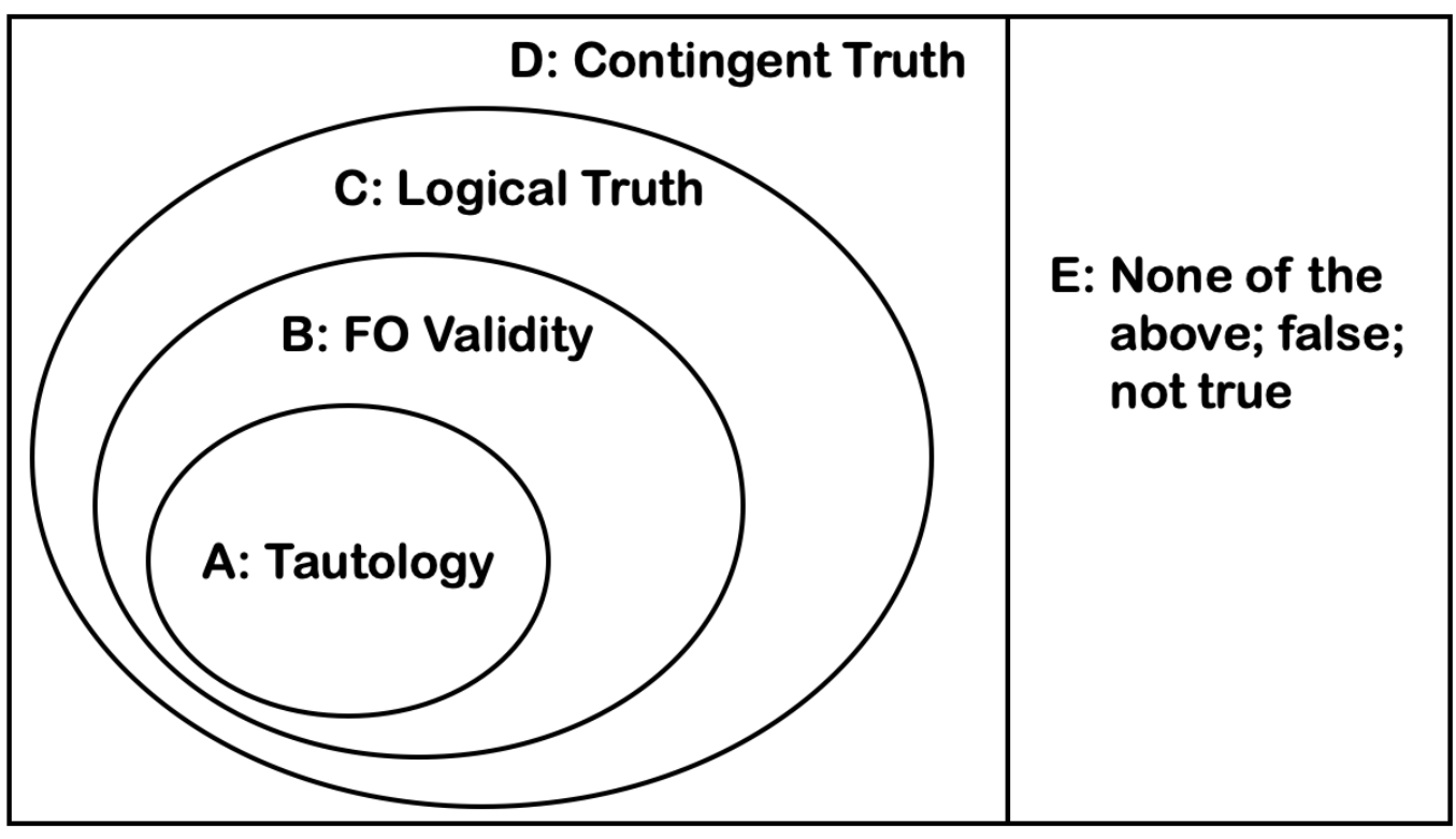
26.4: The Chart

  • We can represent tautologies, FO validites, and logical truths in an Euler diagram.

image


Chapter 27: Counterexamples in FOL

27.1: Counterexamples in FOL

  • Because FOL is not truth functional, we assign meanings to a predicate and names.

Chapter 28: Multiple Quantifiers

28.1: Same Quantifiers

  • Things become more complicated when quantifiers are related to each other and have overlapping scope with multiple binding variables.
  • Somebody likes somebody: \(\exists x \exists y L(x, y)\)
  • Quantifier reorder (QRe): order doesn’t matter.
  • Different quantifiers and variables don’t necessarily pick out different objects
  • Distinctness clauses: \(~(x=y)\)

28.2: Mixed Quantifiers

  • Rule: pick objects for quantifiers from left to right.
  • A sentence is stronger than another if it entails the other, but not vice versa.

Chapter 29: Numerical Quantification

29.1: At Least

  • You need \(n\) existential quantifiers and enough distinctness clauses.
  • The number of distinctness clauses follows the progression of triangular numbers - 1, 3, 6, 10, etc.
  • “There are at least two dogs”: \(\exists x \exists y (D(x)&D(y)&~(x=y))\)

29.2: At Most

  • At most \(n\) means \(n\) or fewer, maybe none.
  • At most \(n\) takes \(n + 1\) universal quantifiers.
  • \[\forall x \forall y \forall z ((D(x) & D(y) & D(z)) \to (x=y \lor x=z \lor y=z))\]
  • The number of equalities is triangular.

29.3: Exactly

  • There are two ways to translate ‘exactly’ into FOL.
  • There are exactly two dogs:
\[\exists x \exists y (D(x) & D(y) & ~x = y) & \forall x \forall y \forall z ((D(x) & D(y) & D9z)) \to (x = y \lor x = z \lor y = z))\] \[\exists x \exists y (D(x) & D(y) & ~x = y & \forall z (D(z) \to (x = z \lor y = z)))\]
  • Short way - ‘exactly \(n\)’ can be translated as \(n\) existential quantifiers and 1 universal.

29.4: Definite Descriptions - ‘The’

  • Definite descriptions imply uniqueness - only one thing can fit the description.
  • Bertrand Russell - logical analysis of definite descriptions to solve the law of the excluded middle.

Chapter 30: Proofs in FOL - 2 Easy Ruels

30.1: Simple Informal Proofs

  • How do steps with qquantifiers work?
  • Universal Instantiation - instantiate general claim in the quantiifer for a specific claim about a particular object.
  • Existential Generalization - how we reason to an existential.

30.2: \(\exists\)Intro - Existential Generalization

  • \(\exists\) Existential Generalization for formal proofs.
  • You can make any claim about an object with any variable.
1. P(a)                 Premise
2. Q(b)                 Premise
3. EyQ(y)               EIntro;2
4. P9a)&EyQ(y)          &Intro;1,3
5. Ex(P(x)&EyQ(y))      EIntro;4

30.3: \(\forall\)Elim - Universal Instantiation

  • In informal proofs, universal instantiation allows you to instantiate a universal quantifier with any name.
  • For \(\forall\) Elim, you must replace every instance of the variable with the same name.

Chapter 31: Proofs in FOL - 2 Hard Rules

31.3: Universal Generalization

  • To reason to a universal claim, we need to use arbitrary names.
  • We assume a temporary name that points towards an arbitrary object and show we can derive a result from that variable.

13.2: \(\forall\) Intro

  • @n: a new symbol to declare an arbitrary symbol.
  • Begin an \(\forall\)Intro proof by putting @a on the assumption line of a new subproof.

13.3: Existential Instantiation

  • We need to be able to reason from an existential.
  • We don’t want to consider a completely arbitrary object in the domain.

13.4: \(\exists\)Elim

  • We begin by assuming an arbitrary name @n.
  • Follow each arbitrary name with a condition upon which we choose an object in the domain.

Chapter 32: = Proofs

23.1: =Elim

  • We can build = into formal proofs.
  • If \(p = a\), we can substitute one name for any other in FOL.
  • =Elim also allows us to substitute one or more occurrences of a name.
  • Transitivity of identity
  • If you want to use multiple different identities, you must do each one step at a time.

23.2: =Intro

  • A logically true conclusion follows from anything.
  • We can introduce a=a any time.
  • Symmetry of identity.

Chapter 33: FOL Proofs

33.1: Universals

  • Quantifiers aren ot connectives. ‘Operator’ - quantifiers and connectives.
  • Look at the main operator.
  • Universal premise: use \(\forall\)Elim; universal conclusion; set up \(\forall\)Intro.
  • Use the name ‘a’ when there are no other names.

33.2: Existentials

  • Existential premise: \(\exists\)Elim.
  • Existential conclusion: look around for other ideas, use \(\exists\)Intro at some point.
  • For existential conclusions, you will often not do \(\exists\)Intro in the last line.
  • Often, \(\exists\)Intro is used within an \(\exists\)Elim subproof.

33.3: Key Pattern ~\(\exists\)xP(x)

  • Negation around a quantifier - provide special challenges.
  • We need to do a reductio built from the inside to handle negation around another connective.
  • When your conclusion is a wide scope \(\forall\)x, begin with an \(\forall\)Intro proof.

33.4: Annoying Pattern ~\(\forall\)xP(x)

  • ~\(\exists\)xP(x) is similar to the five step plan.
  • Indirectly apply the five-step plan using reductio.

33.5: Regular Routine for Quantifiers

  1. Look at the conclusion for a wide-scope universal or negation; if so, start \(\forall\)Intro or ~Intro.
  2. Look for existentials in the premises; if so, start an \(\exists\)Elim proof (existentials before universals).
  3. Instantiate any universals.
  4. Solve proof sets.
  5. Repeat.

Chapter 34: Logic and Set Theory

34.1: Sets and Membership

  • Set - a collection or group of things.
  • Items in a set are members/elements.
  • Sets are abstract collections.
  • We can use universal quantifiers and set-builder notation.
  • Binary predicate for set membership - \(a \in b\). Opposite - \(\notin\).
  • Facts about sets: order doesn’t matter, repetition doesn’t matter, name choice doesn’t matter.
  • Sets can contain other sets.
  • \(\emptyset\) - the empty set.

34.2: Cardinality = Size

  • Every set has a size - cardinality, number of elements in the set.
  • Vertical bars around a set - cardinality of the set.
  • One-to-one correspondence: a way to compare the sizes of two sets.
  • Two sets cannot possibly have different sizes if they can be paired with one-to-one correspondence.

34.3: Natural Numbers and Infinite Sets

  • This textbook is including 0 in the set of natural numbers for some bizarre reason.
  • \(\aleph_0\) - cardinality of the set \(\mathbb{N}\).

34.4: 1-to-1 Correspondence, Transfinite Arithmetic

  • We can do arithmetic with \(\aleph_0\).
  • \[\aleph_0 + 1 = \aleph_0\]

Chapter 35: Logic and Infinity

35.1: E, O, Z

  • \(\mathbb{E}\) - set of even numbers
  • \(\mathbb{O}\) - set of odd numbers
  • \(\mathbb{Z}\) - set of integers.
  • All these sets have the same cardinality as the natural numbers.

35.2: The Rational Numbers Q

  • \(\mathbb{Q}\) - rational numbers - expressed as fractions of whole numbers.
  • Density - between any two numbers, there exists another number.
\[\forall x \forall y \exists z (~(x=y) \to ((x < z & z < y) v (y < z & z < x)))\]
  • Density: means that no two rational numbers are adjacent to each other.
  • We can pair \(\mathbb{Q}\) with \(\mathbb{N}\) as follows: write a table where each column is the numerator and each row is the denominator, then take a snake-coil pattern for the line through the table. Every cell of the table will eventually be covered by the line.
\[\| \mathbb{N} \| = \| \mathbb{Q} \|\]

35.3: The Real Numbers R

  • The reals include the rationals and the irrationals.
  • There are different sizes of infinity - we can prove via reductio that there is no 1-to-1 correspondence between \(\mathbb{R}\) and \(\mathbb{N}\).
  • Cantor’s diagonal argument