Textbook Notes

MATH 126

Table of contents

Chapter 10: Parametric Equations and Polar Coordinates
1. 10.3: Polar Coordinates
Chapter 12: Vectors and the Geometry of Space
Chapter 13: Vector Functions
Chapter 14: Partial Derivatives
Chapter 15: Multiple Integrals

Chapter 10: Parametric Equations and Polar Coordinates

10.3: Polar Coordinates

Polar coordinate system: a point in the plane is the pole. The polar axis is a ray starting from $0$.
Polar coordinates - $(r, \theta)$.
In the polar coordinate system, each point has many representations.

\[\cos \theta = \frac{x}{r}, \sin \theta = \frac{y}{r}\] \[x = r \cos \theta, y = r \sin \theta\] \[r^2 = x^2 y^2; \tan \theta = \frac{y}{x}\]

Polar Curves

Graph of a polar equation - $r = f(\theta)$, or $F(r, \theta) = 0$.
ALl points $P$ with at least one polar representation $(r, 0)$ whose coordinates satisfy the equation.
Symmetry rules
- If a polar equation is unchanged when $\theta$ is negated, the curve is symmetric about the polar axis.
- If the equation is unchanged when $r$ is negated or $\theta$ replaced with $\theta + \pi$, the curve is symmetric about the pole.
- If the equation is unchanged when $\theta$ is replaced with $\pi - \theta$, the curve is symmetric about the vertical line at $\theta = \frac{\pi}{2}$.

Tangents to Polar CUrves

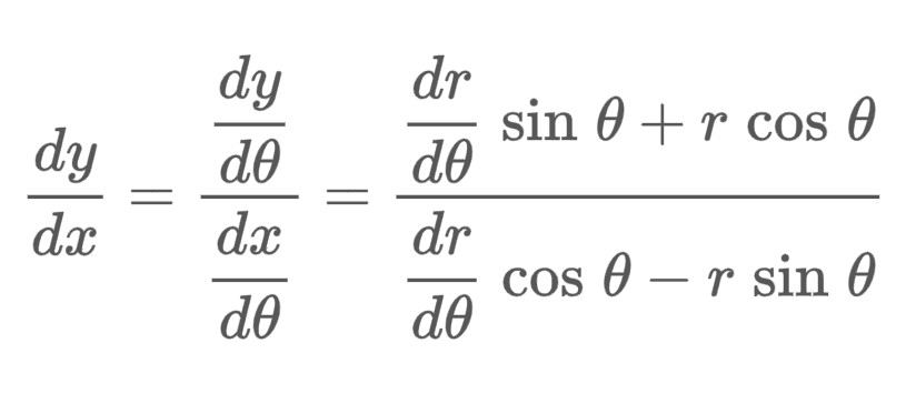
To find the tangent to $r = f(\theta)$, use the following parametric equations:
- $x = f(\theta) \cos \theta, y = f(\theta) \sin theta$.

Chapter 12: Vectors and the Geometry of Space

12.1: Three-Dimensional Coordinate Systems

Three axes form a three-dimensional space.
The three-dimensional space is divided into octants.
If we drop from $P$ to some plane, it is the projection of $P$ onto the $xy$-plane.
The Cartesian product $\mathbb{R} \times \mathbb{R} \times \mathbb{R} = {(x, y, z) \| x, y, z \in \mathbb{R}}$ is the set of all ordered triples of real numbers; denoted $\mathbb{R}^3$.

Surfaces

If $k$ is constant, then:
- $x = k$ represents a plane parallel to the $yz$-plane
- $y = k$ represents a plane parallel to the $xz$-plane
- $z = k$ represents a plane parallel to the $xy$-plane
Circles and cylinders, free restirction over axes

Distance and Spheres

The distance formula $\|P_1P_2\|$ between two points $P_1 (x_1, y_1, z_1)$ and $P_2 (x_2, y_2, z_2)$ is

\[\|P_1P_2\| = \sqrt{(x_2 - x_1)^2 + (y_2 - y_1)^2 + (z_2 - z_1)^2}\]

This formula is a natural extension of the Pythagorean theorem in two dimensions.
The equation of a sphere with center $C$ (h, k, l)$ and radius $r$ is

\[(x - h)^2 + (y - k)^2 + (z - l)^2 = r^2\]

12.2: Vectors

Vector: used to indicate a quantity that has both magnitude and direction. Often represented by an arrow or directed line segment. Vectors are denoted as $\vec{v}$.
A displacement vector $v$ has initial point $A$ and terminal point $B$, which can be notated as $\mathbf{v} = \vec{AB}$.
To combine vectors, simply add the changes.
You can multiply a vector by a scalar $c$.

Components

If we place the initial point of a vector $a$ at the origin of a rectangular coordinate system, the terminal point of $a$ has a coordinate of the form $(a_1, a_2)$ or $(a_1, a_2, a_3)$.
Coordinates are the components of $\mathbf{a}$. We can write these as

\[\mathbf{a} = \langle a_1, a_2 \rangle\] \[\mathbf{a} = \langle a_1, a_2, a_3 \rangle\]

This represents a vector rather than a point.
Different representations of a vector have the same direction and magnitude but may be in different positions. The position with the beginning point at the origin is the posiiton vector of a point.
The magnitude or length of a vector is the length of any of its representations, and is denoted as $\| \vec{v} \|$.
An $n$ dimensional vector is an ordered $n$-tuple.
Basis vectors:
- \[\vec{i} = \langle 1, 0, 0, \rangle\]
- \[\vec{i} = \langle 0, 1, 0, \rangle\]
- \[\vec{i} = \langle 0, 0, 1, \rangle\]
Any vector can be expressed as a linear sum of basis vectors.
Unit vector: a vector whose length is 1. In general if $\vec{a} \neq 0$, then the unit vector that has the same direction as $\vec{a}$ is $\vec{u} = \frac{\vec{a}}{\|\vec{a}\|}$.

Applications

Vectors are useful in many aspects of physics and engineering.
Force is represented by vector because it obht has magnitude and direction.

12.3: The Dot Product

Can we multiply two vectors such that the product is a useful quantity?

If $\vec{a} = \langle a_1, a_2, a_3 \rangle$ and $\vec{b} = \langle b_1, b_2, b_3 \rangle$, then the dot product $\vec{a} \cdot \vec{b}$ is

\[\vec{a} \cdot \vec{b} = a_1 b_1 + a_2 b_2 + a_3 b_3\]

The result of a dot product is not a vector, but a scalar. The dot produce is sometimes called the scalar product or inner product.
Properties of the dot product:
1. $$\vec{a} \cdot \vec{a} = |\vec{a}|^2
2. \[\vec{a} \cdot \vec{b} = \vec{b} \cdot \vec{a}\]
3. \[0 \cdot \vec{a} = 0\]
4. \[\vec{a} \cdot (\vec{b} + \vec{c}) = \vec{a} \cdot \vec{b} + \vec{a} \cdot \vec{c}\]
5. \[(c\vec{a}) \cdot \vec{b} = c(\vec{a} \cdot \vec{b}) = \vec{a} \cdot (c\vec{b})\]
The dot product can be interpreted in terms of the angle between $\vec{a}$ and $\vec{b}$:

If $\theta$ is the angle between the vectors $\vec{a}$ and $\vec{b}$, then

\[\vec{a} \cdot \vec{b} = \|\vec{a} \| \| \vec{b} \| \cos \theta\]

If $\theta$ is the angle between the nonzero vectors $\vec{a}$ and $\vec{b}$, then

\[\cos \theta = \frac{\vec{a} \cdot \vec{b}}{\| \vec{a} \| \| \vec{b} \|}\]

Two nonzero vectors are perpendicular/orthogonal if the angle between them is $\theta = \frac{\pi}{2}$. Two nonzero vectors ar eorthogonal if and only if their dot product is 0.

Direction Angles and Direction Cosines

Direction angles of a nonzero vector are the angles $\alpha, \beta, \gamma$ that a vector makes with the positive axes.
The cosines of the direction angles are the direction cosines.

\[\cos \alpha = \frac{a_1}{\|\vec{a}\|}\] \[\cos \beta = \frac{a_2}{\|\vec{a}\|}\] \[\cos \gamma = \frac{a_3}{\|\vec{a}\|}\]

We can square expressions and see the following:

\[\cos^2 \alpha + \cos^2 \beta + \cos^2 \gamma = 1\]

We can also write the following:

\[\vec{a} = \langle a_1, a_2, a_3 \rangle = \langle \| \vec{a} \| \cos \alpha, \| \vec{a} \| \cos \beta, \| \vec{a} \| \cos \gamma \rangle = \| \vec{a} \| \langle \cos \alpha, \cos \beta, \cos \gamma \rangle\]

Dividing both sides by $\| \vec{a} \|$, we see that the direction cosines of $\alpha$ are the components of the unit vector in the direction of $\vec{a}$.

Projections

Consider $\vec{PQ}$ $\mathbf{a}$ and $\vec{PR}$ $\mathbf{b}$ with the same initial point $\vec{P}$. If $S$ is the foot of the perpendicular from $R$ to the line containing $\vec{PQ}$, then the vector with representation $\vec{PS}$ is the vector projection of $\mathbf{b}$ onto $\mathbf{a}$, denoted by $\text{proj}_a \mathbf{b}$.
- Think of this as the shadow of $\mathbf{b}$.
Scalar projbection of $\mathbf{b}$ onto $\mathbf{a}$ (the component of $\mathbf{b}$ along $\mathbf{a}$) is the signed magnitude of the vector projection, which is $\| \mathbf{b} \| \cos \theta$, where $\theta$ is the angle between $\mathbf{a}$ and $\mathbf{b}$. This is denoted as $\text{comp}_a \mathbf{b}$; this is negative if $\frac{\pi}{2} < \theta \le \pi$.

\[\mathbf{a} \cdot \mathbf{b} = \| \mathbf{a} \| \| \mathbf{b} \| \cos \theta = \| \mathbf{a} \| (\| \mathbf{b} \| \cos \theta )\]

The dot product of two vectors can be interpreted as the length of one multiplied by the scalar projection of the other vector upon the first vector.

Calculating work

The work done by a constant force $\vec{F}$ is $\vec{F} \cdot \vec{D}$, where $\vec{D}$ is the displacement vector.

12.4: The Cross Product

Given two nonzero vectors, it is very useful to find a nonzero vector that is perpendicular to both vectors.
The cross product of $\vec{a} = \langle a_1, a_2, a_3 \rangle$ and $\vec{b} = \langle b_1, b_2, b_3 \rangle$ is

\[\vec{a} \times \vec{b} = \langle a_2 b_3 - a_3 b_2, a_3 b_1 - a_1 b_3, a_1 b_2 - a_2 b_1 \rangle\]

The cross product/vector product is only defined when $\vec{a}$ and $\vec{b}$ are three-dimensional.
Determinant interpretation of the cross-product.
The vector $\vec{a} \times \vec{b}$ is orthogonal to both $\vec{a}$ and $\vec{b}$.
The right-hand rule gives the direction of $\vec{a} \times \vec{b}$.
If $\theta$ is the angle between $\vec{a}$ and $\vec{b}$, then $\| \vec{a} \times \vec{b} \| = \| \vec{a} \| \| \vec{b} \| \sin \theta$.
Geometric characterization: $\vec{a} \times \vec{b}$: a vector perpendicular both to $\vec{a}$ and $\vec{b}$.
Two nonzero vectors $\vec{a}$ and $\vec{b}$ are parallel if and onlny if $\vec{a} \times \vec{b} = 0$.
The length of the crossproduct $\vec{a} \times \vec{b}$ is equal to the area of the parallelogram formed by $\vec{a}$ and $\vec{b}$.
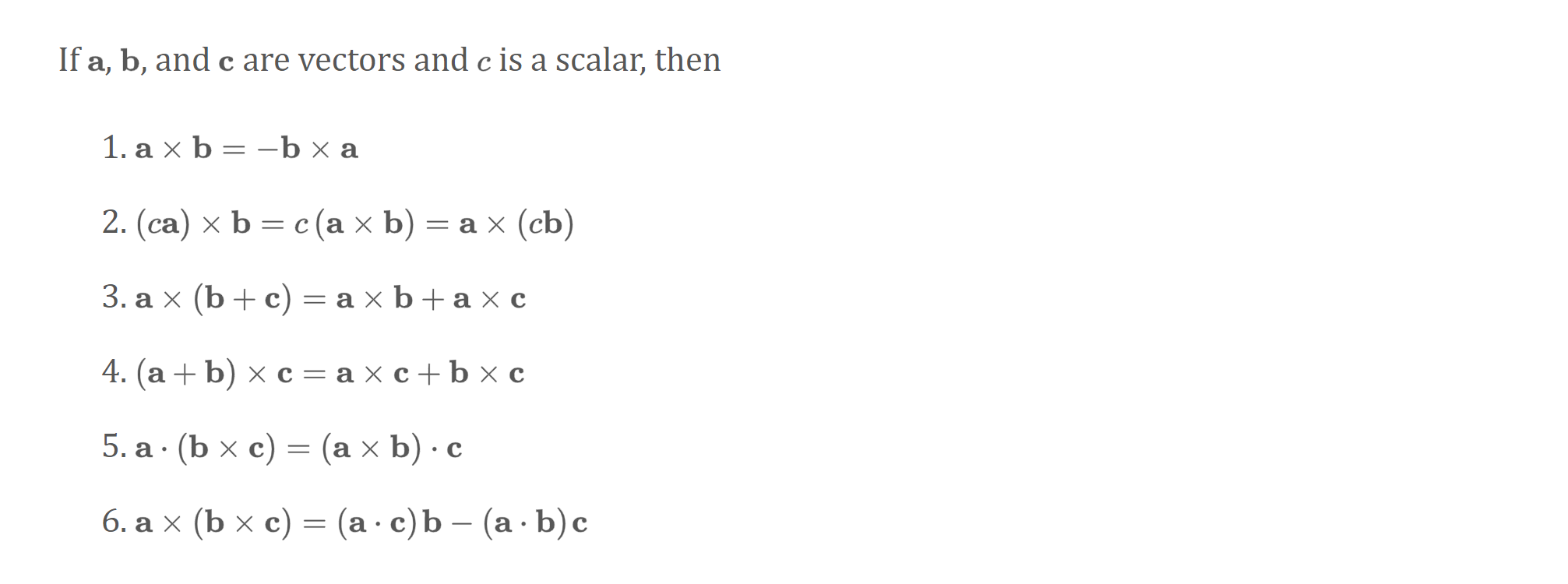
The cross-product is not commutative. $\vec{i} \times \vec{j} \neq \vec{j} \times \vec{i}$. The associative law does not hold either.

Triple Products

The product $\vec{a} \cdot (\vec{b} \times \vec{c})$ - scalar triple product of the vectors $\vec{a}$, $\vec{b}$, and $\vec{c}$.
Parallelepiped volume $V$ is the magnitude of the scalar triple:

\[V = Ah = \| \vec{b} \times \vec{c} \| \| \vec{a} \| \| \cos \theta \| = \| \vec{a} \cdot (\vec{b} \times \vec{c} ) \|\]

If the scalar product is 0, the vectors lie on the same plane and are coplanar.

12.5: Equations of Lines and Planes

Let $P(x, y, z)$ be an arbitrary point on a line $L$. Let $\vec{r}_0$ and $\vec{r}$ be the position vectors of $P_0$ and $P$. The following is true for some vector $\vec{a} = \vec{P_0 P}$ and some scalar $t$.

\[\vec{r} = \vec{r}_0 + t \vec{v}\]

This is the vector equation of the line.

We can expand the vector equation of a line, and we obtain the parameteric equations derived from identifying the components of the result of the vector equation.

\[x = x_0 = at\] \[y = y_0 + bt\] \[z = z_0 + ct\]

The vector equation and parameteric equations of a line are not unique; we can change the point, parameter, or choose a different parallel vector. This will change the line.

Symmetric equations: derived from solving each of the parameter equations for $t$, then setting the expressions all equal to each other.
You can set a limitation on $t$ to express only a certain line segment.
The line segment from $\vec{r}_0$ to $\vec{r}_1$ is given by the vector equation

\[\vec{r} = (1 -t ) \vec{r}_0 + t \vec{r}_1, 0 \le t \le 1\]

A plane in space is more difficult to describe. A plane in space is determined by a point $P_0$, a vector $\vec{n}$ orthogonal to the plane. Let $\vec{r}_0$ and $\vec{r}$ be the position vectors of $P_0$ and $P$. $\vec{r} - \vec{r}_0$ is orthogonal to $\vec{n}$.

\[\vec{n} \cdot (\vec{r} - \vec{r}_0) = 0 \implies \vec{n} \cdot \vec{r} = \vec{n} \cdot \vec{r}_0\]

Scalar equation for the plane: write

\[\vec{n} = \langle a, b, c \rangle\] \[\vec{r} = \langle x, y, z \rangle\] \[\vec{r}_0 = \langle x_0, y_0, z_0 \rangle\]

This simplifies into

\[a (x - x_0) + b(y - y_0) + c(z - z_0) = 0\]

We can rewrite the equation as such:

\[ax + by + cz + d = 0\]

Here, $d = -(ax_0 + by_0 + cz_0)$. This is the linear equation in $\mathbb{R}^3$.

12.6: Surfaces

Cylinders and quadric surfaces.
Traces/cross-sections - curves of intersection on the surface with planes paralle to the coordinate planes.

Cylinders

Consists of all lines that are parallel to a given line and pass through a given plane curve.
Parabolic cylinder - made up of infinitely many shifted copies of the same parabola.

Quadric Surfaces

A quadric surface is the graph of a second degree equation in three variables.

\[Ax^2 + By^2 + Cz^2 + Dxy + Eyz + Fxz + Gx + Hy + Iz + J = 0\]

To sketch an image, find how traces scale in each dimension.

Chapter 13: Vector Functions

13.1: Vector Functions and Space Curves

Vector-valued function/vector function: a function whose domain is a set of real numbers and whose range is a set of vectors.
Each number $t$ in the domain of $\mathbf{r}$ has a unique vector in $\mathbf{V}_3$.
If $\{f(t), g(t), h(t)}$ are components of the vector $$\mathbf{r}44, we have:

\[\mathbf{r}(t) = \langle f(t), g(t), h(t) \rangle = f(t) \vec{i} + g(t) \vec{j} + h(t) \vec{k}\]

Limits and Continuity.

The limit of a vector function is defined by taking the limits of the component functions.

\[\lim_{t\to a} \mathbf{r}(t) = \langle \lim_{t\to a} f(t), \lim_{t\to a} g(t), \lim_{t\to a} h(t) \rangle\]

Taking the limit can be interpreted as saying that the length and direction of the vector $\mathbf{r}$ approach the length and direction of the vector $\vec{L}$ (where $\vec{L}$ is the result of the limit.
A vector function is continuous at $a$ if $$\lim_{t\to a} \mathbf{r}(t) = \mathbf{r}(a)44.
- The component functions of a vector function must all be continuous at $a$ for the vector function itself to be considered continuous at $\vec{a}$.

Space curves.

Set $C$ of all points $(x, y, z)$ with $x = f(t), y=g(t), z = h(t)$, the space curve is derived by tracing $t$ through an interval $I$.
The equations are the parametric equations of $C$; $t$ is the parameter.
Any continuous vector defines space curve $C$ traced out by moving the tip of the moving vector $\mathbf{r}(t)$.
Plane curves can be represented in vector notation. The curve given by the parametric equations $x = t^2 - 2t$ and $y = t + 1$ can be described via

\[\mathbf{r}(t) = \langle t^2 - 2t, t + 1 \rangle\]

Helix: given by $x = \cos t, y = \sin t, z = t$

13.2: Derivatives and Integrals of Vector Functions

Derivatives.

The derivative of a vector function $\mathbf{r}$ is dfined similarly for real-valued functions. Take the derivative of the element-wise component functions.
The second derivaitv eof avector function is the derivative of $\mathbf{r}$.

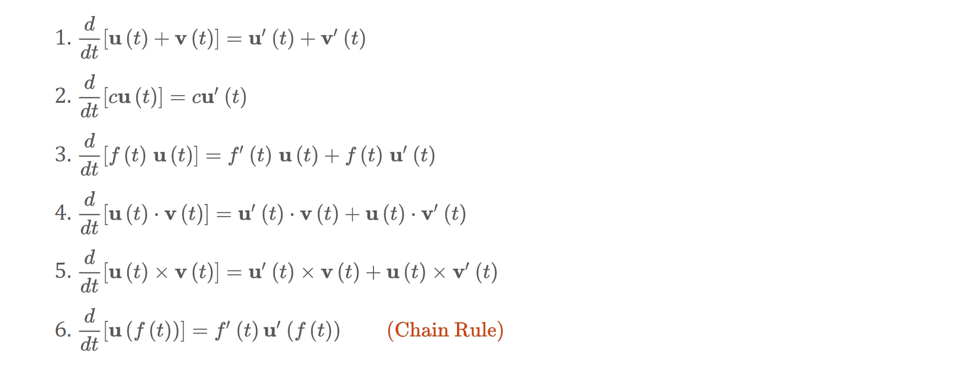
Differentiation Rules

Differentiation formulas for real-valued functions have counterparts for vector-valued functions.

Integrals.

You can integrate component-wise, like normal.

13.3: Arc Length and Curvatutre

\[L = \int_a^b \int{f'(t)^2 + g'(t)^2 + g'(t)^2}\] \[L = \int_a^b \| r'(t) \| dt\]

$r(t)$ is the position vector, $r'(t)$ is the velocity vector, $\| r'(t) \|$ is the speed. To compute distance traveled, integrate speed.

The Arc Length Function

Arc length function $s$: defined as follows for some $a$:

\[s(t) = \int_a^t \| \vec{r}'(u) \| du\]

We see that $\frac{ds}{dt} = \| \vec{r} '(t) \|$
It is useful to parametrize a curve w.r.t. arc length - arc length arises naturally from the curve shape and is not coordinate-dependent.
- Solve for $t$ as a function of $s$, then reparametrize in terms of $s$.

Curvature

A parametrization is smooth on an interval if the derivative is continuous and $\vec{r}'(t) \neq 0$. A curve is smooth if it has a smooth parametrization. Smooth curves have no sharp corners; the tangent vector turns continuously.
Curvature - measure of how quickly the curve changes direction.
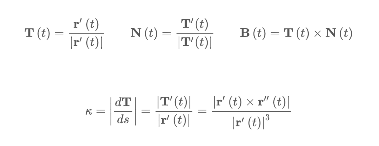
The curvature of a curve is $\| \frac{d\vec{T}}{ds} \| = \| \frac{\vec{T}'(t)}{\vec{r}'(t)} \|$, where $\vec{T}$ is the unit tangent vector.
The curvature of the curve given by a vector function $\vec{r}$ is

\[\frac{\| \vec{r}'(t) \times \vec{r} ''(t) \|}{\| \vec{r}'(t) \| ^3}\]

The Normal and Binormal Vectors

Many vectors are orthogonal to the unit tangent vector $\vec{T}(t)$. Note that $\vec{T}(t) \cdot \vec{T}'(t) = 0$, so $\vec{T}'(t)$ is orthogonal to $\vec{T}(t)$.
At any point where $\kappa \neq 0$, we can define the principal unit normal vector/unit normal vector $\vec{N}(t) = \frac{\vec{T}'(t)}{\| \vec{T}'(t) \|$.
The unit normal vector indicates the direction in which the curve is turning at each point.
$\vec{B}(t) = \vec{T}(n) \times \vec{N}(t)$ - binormal vector. Is a unit vector orthogonal to $\vec{T}(t)$ and $$\vec{N}(t)44.
Normal plane - plane spanned by the normal and binormal vectors. Consists of all lines orthogonal to the tangent line
Osculating plane spanned by $\vec{T}$ and $\vec{N}$. Plane that comes closest to containing the part of the curve near $\vec{P}$.
Osculating circle/circle of curvature of $C$ at $P$. Shares the same tangent, normal, and curvature at $P$.

13.4: Motion in Space

Tangent and normal vectors can be used in physics to study velocity and acceleration along a space curve.
Velocity vector $\vec{v}(t) = \vec{r}'(t)$.
Speed is the magnitude of the velocity vector.
Acceleration is the derivative of velocity: $\vec{a}(t) = \vec{v}'(t)$.
Vector integrals allow us to recover velocity when acceleration is known and position when velocity is known.

\[\vec{v}(t) = \vec{v}(t_0) + \int_{t_0}^t \vec{a}(u) du\] \[\vec{r}(t) = \vec{r}(t_0) + \int_{t_0}^t \vec{v}(u) du\]

Newton’s Second Law of Motion: a force $\vec{F}(t)$ acts on an object of mass $m$ produces an acceleration $\vec{a}(t)$. The following is true:

\[\vec{F}(t) = m\vec{a}(t)\]

Tangent and Normal Components of Acceleration

Acceleration can be separated into the direction of the tangent and the direction of the normal.

$\vec{a} = a_T \vec{T} + a_n \vec{N}; a_T = v', a_N = \kappa v^2$$

Acceleration always lies on the plane of $\vec{T}$ and $\vec{N}$, the osculating plane.
The tangential component of acceleration is $v'$ (derivative of speed); the normal component is $\kappa v^2$, or curvature tiems speed squared.

\[a_T = v' = \frac{\vec{r}'(t) \dot \vec{r}''(t)}{\| \vec{r}'(t) \|}\] \[a_N = \frac{\vec{r}'(t) \times \vec{r}''(t) \| }{\| \vec{r}'(t) \|}\]

Chapter 14: Partial Derivatives

14.1: Functions of Two Variables

A function of two variables is a rule that assigns an ordered pair of real numbers to a unique real number: $R = {f(x, y) \| (x, y) \in D}$.
Linear functions of two variables are important in multivariable calculus.
Level curves: curves satisfying $f(x, y) = k$ for some constant $k \in R$.
A function of three variables maps points in $\mathbb{R}^3$ to a real number.
A function of $n$ variables: maps an $n$-tuple within $\mathbb{R}^n$ to a real number.

14.2: Limits and Continuity

Let $f$ be a function of two variables; the limit of $f(x, y)$ as $(x, y)$ approaches $(a, b)$ is $L$:

\[\lim_{(x, y) \to (a, b)} f(x, y) = L\]

We can let $(x, y)$ approach $(a, b)$ from an infinite number of directions (as opposed to just two in one dimension).

If $f(x, y) \to L_1$ as $(x, y) \to (a, b)$ along a path $C_1$ and If $f(x, y) \to L_2$ as $(x, y) \to (a, b)$ along a path $C_12$ with$L_1 \neq L_2$, then the limit$\lim_{(x, y) \to (a, b)} f(x, y)$$ does not exist.

Continuity

A function of two variables is continuous at $(a, b)$ if $\lim_{(x, y) \to (a, b)} f(x, y) = f(a, b)$. $f$ is continuous on $D$ if $f$ is continuous at every point $(a, b)$ in $D$.
If the point $(x, y)$ changes, then the value of $f(x, y)$ changes by a small amount: there is no hole or break.
Polynomial function of two variables - sum of terms in $c^my^n$.
Rational function: a ratio of polynomials.
All polynomials and rtional functions are continuous on their domains.

Functions of 3+ variables

Everything can be expanded two three or more dimensions.
If $f$ is defined on a subset $D$ of $\mathbb{R}^n$, then $\lim_{x\to a} f(x) = L$ means that for every number $\epsilon > 0$, there is a corresponding number $\delta > 0$ such that if $x \in D$ and $0 < \| x - a \| < \delta$ then $\| f(x) - L \| < \epsilon$.

\[\lim_{x\to a} f(x) = f(a)\]

14.3: Partial Derivatives

The partial derivative of a function with respect to $x$ at $(a, b)$ is denoted $f_x(a, b)$. Thus, $f_x(a, b) = g'(a)$ where $g(x) = f(x, b)$.
The partial derivative of $f$ with respect to some variable at $(a, b)$ is obtained by fixing other variables and finding the ordinary derivative at $b$ of the fixed function.

\[f_x(x, y) = \lim_{h\to 0} \frac{f(x+h, y) - f(x, y)}{h}\]

Alternative notation: $\frac{\alpha f}{\alpha x}$
To find $f_x$, treat $y$ as a constant and differentiate w.r.t. $x$. Vice versa for $f_y$.

Interpretations of Partial Derivatives

By fixing other dimensions at a constant, we restrict attention to the curve at which a hyperplane intersects the surface.
In two dimensions, $f_x(a, b)$ and $f_y(a, b)$ an be interpreted as the slopes of the tangent lines at $P(a, b, c)$ to the traces $C_1$ and $C_2$ of the surface $S$ in the planes $y=b$ and $x=a$.
$\alpha z / \alpha y$ is the rate of change in $z$ with respect to $y$ when $x$ is fixed for some function $z = f(x, y)$.

Higher Derivatives

We can compute higher-order partial derivatives:

\[(f_x)_x = f_{xx} = f_{11} = \frac{\alpha}{\alpha x} \left( \frac{\alpha f}{\alpha x} \right) = \frac{\alpha^2 f}{\alpha x^2}\]

Clairaut’s Theorem. Suppose $f$ is defined on a disk $D$ tht contains the point $a, b$. If the functions $f_{xy}$ and $f_{yz}$ are both continuous on $D$, then $f_{xy}(a, b) = f_{yz} (a, b)$.

Partial Differential Equations

Laplace’s equation: $\frac{\alpha^2 u}{\alpha x^2} + \frac{\alpha^2 u}{\alpha y^2} = 0$
Harmonic functions are solutions to Laplace’s equation.
3-dimensional Laplace equation: $\frac{\alpha^2 u}{\alpha x^2} + \frac{\alpha^2 u}{\alpha y^2} + \frac{\alpha^2 u}{\alpha z^2} = 0$
Wave equation: $\frac{\alpha^2 u}{\alpha t^2} = a^2 \frac{\alpha^2 u}{\alpha x^2}$

Differentials

We can define the differential to be an independent variable.
Differential of $y$ is $dy = f'(x) dx$
For a differentiable function of two variables, we can define $dx$ and $dy$ to be independent variables. The total differential $dz$ is

\[dz = f_x(x, y) dx + f_y(x, y) dy = \frac{\partial z}{\partial x} dx + \frac{\partial z}{\partial y} dy\]

$$f(x, y) \approx f(a, b) + dz44

14.4: Tangent Lines and Linear Approximations

We can extend the tangent line to approximate values near a point.

Tangent Planes

The tangent plane to the surface $S$ at point $P$ is the plane containing both tangent lines.

\[z - z_0 = a(x - x_0) + b(y - y_0)\] \[a = f_x(x_0, y_0), b = f_y(x_0, y_0)\]

Linear Approximations

Linearization $L$: a linear approximation/tangent plane approximation of a function $f$ at some point $P$.

\[\Delta y = f'(a) \Delta x + \epsilon \Delta x, \epsilon \to 0 \text{ as } \Delta x \to 0\]

14.7: Maximum and Minimum Values

If $f$ has a local maximum or minimum at $(a, b)$ and the first-order partial derivatives of $f$ exist there, then $f_x(a, b) = 0$ and $f_y(a, b) = 0$.
Critical point/stationary point: if both partial derivatives are 0 or one of them does not exist.
Second derivative test - find $D$ as follows.

\[D(a, b) = f_{xx}(a, b) f_{yy}(a, b) - \[f_{xy} (a, b)\]^2\]

If $D > 0$, then $f(a, b)$ is a local minimum or maximum.
If $f_{xx}(a, b) > 0$, then local minimum.
If $f_{xx}(a, b) < 0$, then local maximum.
If $D < 0$, then not a local maximum or minimum (saddle point).
If $D = 0$, then inconclusive.

Absolute Maximum and Minimum Values

Extreme Value Theorem - if $f$ is continuous on a closed interval ${a, b]$, then $f$ has an bsolute minimum and maximum value.
A closed set contains all of its boundary points.
A bounded set is ‘finite’.
To find the absolute minimum and maximum values, find the critical points, find the extreme values on the boundary, and find the largest and smallest values from these sets.

Chapter 15: Multiple Integrals

15.1: Double Integrals over Rectangles

We can find the volume of a solid with double integrals.
We can consider a function of two variables defined on a closed rectangle $R = [a, b] \times [c, d]$.

The double integral of $f$ over the rectangle $R$ is

$\int \int_R f(x, y) dA = \lim_{m, n \to \infty}$ \sum^m_{i=1} \sum^n_{j=1} f(x_{ij}^, y_{ij}^) \Delta A$$

Double Riemann sum: approximation of a Riemann sum.
Methods using for approximating single integrals have parallels in double integrals.
Midpoint Rule for double integrals
Iterated integrals
Partial integration (similar to partial differentiation): treat the inside integral as a function and integrate.
Iterated integral: $\int_a^b \int_c^d f(x, y) dy dx$; integrate $y$ from $c$ to $d$, then $x$ from $a$ to $b$.
Fubini’s theorem:

\[\int_a^b \int_c^d f(x, y) dy dx = \int_c^d \int_a^b f(x, y) dx dy\]

15.2: Double Integrals over General Regions

For single integrals, we always integrate over an interval.
For double integrals, we want to integrate a function over regions of a general shape $D$.
Function $F$: $f(x, y)$ if $(x, y)$ is in $D$ and $0$ if in a rectangle $R$ but not in $D$.
Double integral of $f$ over $D$:

\[\int \int_D f(x, y) dA = \int \int_R F(x, y) dA\]

Type 1 plane region: lies between the graphs of two continuous functions of $x$.
Choose a rectangle $R = [a, b] \times [c, d]$ that contains $D$. By Fubini’s theorem, we have

\[\int \int_D f(x, y) dA = \int_a^b \int_c^d F(x, y) dy dx\]

Type II: oriented in the other direction; express instead by integrating w.r.t. $y$.

Properties of Double Integrals

*The following is true if $f(x, y) \ge g(x, y)$4 for all$(x, y)44 in $D$.

Given $D = D_1 \union D_2$ and $D_1$ does not overlap with $D_2$, then the following is true:

15.3: Double Integrals in Polar COordinates

Suppose we want to evaluate a double integral on a circular region. It is difficult to integrate in a Euclidean system, but easier using polar coordinates.
If $f$ is continuous on a polar rectangle $R$ given by $0 \le a \le r \le b$, $\alpha \le \theta \le \beta$, where $0 \le \beta - \alpha \le 2 \pi$, then

\[\int \int_R f(x, y) dA = \int_\alpha^\beta \int_a^b f(r \cos \theta, r \sin \theta ) r dr d \theta\]

We have $x = r \cos \theta, y = r \sin \theta$.
If $f$ is continuous on a polar region of the form $$D = {(r, \theta) \alpha \le \theta \le \beta, h_1 (\theta) \le r \le h_2 (\theta )}$$.

15.4: Applications of Double Integrals

Density and Mass

We can approximate the mass of an object by integrating over the surface.
We can measure total charge by integrating over the individual charges at each instance.

Moments and Centers of Mass

We can consider a lamina with uniform density using double integrals.

\[M_x = \int \int_D y \rho (x, y) dA\] \[M_y = \int \int_D x \rho (x, y) dA\] \[\bar{x} = \frac{M_y}{m}, \bar{y} = \frac{M_x}{m}\] \[m = \int \int_D \rho (x, y) dA\]

Moment of Inertia

Second moment/moment of inertia: $mr^2$, where $m$ is the pass of the particle and $r$ is the distance from the particle to the axis.
Apply to a lamina with density function $\rho(x, y)$.

Moment of inertia of the lamina about the $x$-axis:

\[I_x = \int \int_D y^2 \rho(x, y) dA\]

Moment of inertia of the lamina about the $y$-axis:

\[I_y = \int \int_D x^2 \rho(x, y) dA\]

Moment of inertia of the lamina about the origin/polar moment of inertia:

\[I_0 = \int \int_D (x^2 + y^2) \rho(x, y) dA\] \[I_0 = I_x + I_y\]